Bioaeroelastic linear stability analysis and
nonlinear time simulations
Pilot-vehicle system bond graph
Bond graphs for a structural modeling approach
From the bond graph models of both helicopter and pilot developed in the previous chapters, one can assemble them into one graph as illustrated on Figure 4-2. In the Cartesian space this is equivalent to what can be seen on Figure 4-1, where the point P1 is the center of the spherical joint between the pilot’s arm and the cockpit of the helicopter. The points P2 to P9 are attachment points of muscles between the pilot and the cockpit. The implicit assumption made here is that the pilot’s torso cannot move in the seat and the seat cannot move either with respect to the cockpit. Interestingly, one can see the points that appear in the physical space are materialized at the bond graph level see Figure 4-1 and Figure 4-2. The frontiers of the system’s subsystems are explicitly represented, and the physical quantity that is exchanged between them is power. This is why the bond graph method is said to be structural (Chikhaoui, 2013); in other words, the global bond graph of a complex system can be decomposed into sub graphs that have the same frontiers as the physical subsystems. The power exchanged between the pilot arm and the helicopter airframe through the point P1 is the result of the product of both static and kinematic screws16 PP arm P arm P arm arm F V M Ω (60) The green and purple arrows behind P1 on Figure 4-2 respectively transport the force-velocity and the angular velocity-moment products. For the rest of the points Pi of Figure 4-1 for i between 2 and 9, the power exchanged expression is, , /0 . P Muscle i airframe P airframe i i P F V (61) This quantity is materialized on the graph Figure 4-2 by the green arrow behind each Pi point (for i between 2 and 9)
Pilot biodynamics model order reduction
The pilot biodynamics model developed in the previous chapter can be used in several manners. The first one consists in directly analyzing the resulting bioaeroelastic model developed previously for which several flight conditions and cabin configurations could be virtually simulated and explored. A second approach, consists in coupling a given vehicle model with a pilot model obtained by identification from experimental results or numerical simulation results, see Figure 4-4. In order to see how the involuntary pilot behavior can affect the stability of a helicopter on its lateral-roll axis, it is proposed to use the second approach and to perform a sweep of potential pilot neuromuscular system’s behaviors for a given helicopter. Furthermore, in order to be able to use powerful stability analysis tools such as Lyapunov’s indirect method (eigenvalue analysis of dynamic system’s state space matrix) and Campbell diagrams17, the pilot model is proposed to be reduced to a second order model, as follows, 2 2 2 . ( ) 2. . . lat k bdft s x s s (62) It also allows reducing the computational cost and more importantly to give the possibility to sweep a wide range of potential involuntary pilot behaviors. On Figure 4-3, the experimental results come from (Venrooij, et al., 2011) on the top of what, the numerical simulations results (LSA – least squares approximation) of the previous chapters have been superposed. The three model reductions presented on the same figure represent three different pilot neuromuscular model setups for which the gain k and the resonant frequency ω of the transfer function on equation (62) vary: the higher these parameters are, the ‘stiffer’ one could qualify the pilot involuntary behavior. These are the same quantities that are swept over a wide range of value on Figure 4-5.
Lateral-roll axis linear stability analysis and nonlinear time simulations
In this section, the models developed previously are analyzed, in particular on the lateral-roll axis of the helicopter. First a linear model is analyzed and then nonlinear time simulations are carried out. 4.2.1.Linear stability analysis results The linearized equations from the vehicle model could have been obtained from the bond graph and would give the same results than the state space model that we have derived using Lagrange equations on section 2.2.3 Lateral/roll dynamics validity of the model around hover. The pilot model is concatenated to the helicopter model by first expressing the transfer function of equation (62) in the time domain, which becomes, 1 1 2 2 1 2 0 G G k G c c c x (63) Where the parameter G corresponds to kinematic ratio between the maximum cyclic blade pitch angle and cyclic lever roll angle, lat c G 1 . Then equation (63) is added to M, C and K matrices, see Appendix 2, with 1c as an additional state variable. The resulting system can put into the state space form,x = Ax (64) With the state vector x= [q̇ , q] T , and the generalized coordinates vector q, 0 1 1 0 1 1 1 , , , , , , , , , T y c s c s c x z q The stability of the equilibrium of the bioaeroelastic system can then be assessed by computing the real part of the eigenvalues of the state space matrix A. As mentioned previously, literature works (Muscarello, et al., 2015) have conjectured the potential mode that can be destabilized due to pilot BDFT is the regressing lag mode as in 115 ground resonance phenomena18. The approach presented here proposes a model that proves this conjecture. Furthermore, the results show that not only the regressing lag mode can be destabilized by the pilot involuntary behavior, but also the progressive lag mode, see Figure 4-5. A set of parameters is fixed for the helicopter and the pilot, see Table 3. These parameters correspond to a medium weight helicopter; the individual blade lag motion natural frequency δ is inferior to the rotor angular velocity, 1.53 0.33 bl k Hz I The positioning of δ corresponds to a soft-in-plane rotor technology (δ<Ω) and has lightly damped in-plane rotor modes, see Figure 2-22. Actually there are two very important instabilities that can develop in soft-in-plane rotor technologies with lightly damped modes which are the ground and air resonance (Krysinski & Malburet, 2011). On Figure 4-5, the real part of the eigenvalues of both regressing and advancing lag modes have been computed for varying values of potential pilot neuromuscular system settings. On those figures it is interesting to notice that the instability domains do not have the same shape and in particular that for a pilot resonant frequency above around 3Hz (~ Ω-δ ) the regressing lag mode recovers more and more damping even if the pilot’s neuromuscular system ‘stiffens’