Many different kinds of heterogeneities can be found within polycrystals such as metallurgical phases, grains morphology, inclusions, residual stresses, crystal anisotropy, etc. These heterogeneities are responsible for local stress concentrations that can lead to early crack initiations. The random character of heterogeneities makes difficult to evaluate their impact on materials fatigue life and thus requires a systematic statistical study. Performing experimentally a statistical analysis of a material fatigue life is expensive and time-consuming. For that reason, predictive tools are of significant interest.
Several numerical models exist to predict materials stress-fields which can be roughly divided into two groups: the full-field models that are accurate but computationally expensive and the mean-field models that are fast and efficient but sometimes lack of accuracy. In order to capture the full range of the stress heterogeneities within a material, all the microstructural heterogeneities must be considered, which are often disregarded by mean-field models, and a very large number of configurations of heterogeneities must be studied, which is too much time consuming with full-field models.
In order to accelerate the computation time, approximations are necessary and some heterogeneities have to be ignored. A phenomenon that is often disregarded is the grains stress variations in polycrystals due to their close environment mechanical properties, the so-called neighborhood effect. This phenomenon can generate large stress concentrations that must be predicted for a better understanding of fatigue damage. This work is an attempt to develop an analytical model with the purpose to quantify polycrystals micromechanical behavior accounting for the neighborhood effect based on simplifying assumptions for a low computational cost in order to study a large amount of heterogeneities distributions.
Introduction to material fatigue
For several decades, fatigue, phenomenon responsible for mechanical parts breakage, has raised a large number of studies combining industrial and scientific expertise. According to the ASTM (Ame, 1997), material fatigue is “the process of progressive localized permanent structural change occurring in a material subjected to conditions that produce fluctuating stresses and strains at some point (or points) and that may culminate in cracks or complete fracture after a sufficient number of fluctuations”. These conditions can be of different kinds (mechanical, thermal, chemical, etc.), and mechanical loads are the sources of fluctuations studied within the framework of this thesis. Depending on the stress amplitude, these cracks can lead on the long term to the material failure without any apparent damage. The basics and generalities of metal fatigue are presented in this section. For more details on the subject, the reader is invited to consult Krupp (2007), Hertzberg, Vinci & Hertzberg (2012) and Bathias & Pineau (2013) books.
Materials fatigue life is generally studied by means of a fatigue test which consists of cyclically loading the part at a constant stress or strain amplitude until failure. From these tests are drawn the SN-curve, which represents the stress amplitude as a function of the number of cycles necessary to fail the component . This curve can be divided in 3 domains:
– Low Cycle Fatigue (LCF) corresponds to stress amplitude close or above the material yield strength. Plasticity plays the most significant role and can be observed visibly. Cracks initiate quickly and failure occurs generally at the surface after a low number of cycles (N < 10⁵ ).
– High Cycle Fatigue (HCF) corresponds to stress amplitude below the material yield strength. Plasticity is macroscopically low or nonexistent but still exists at the microscopic scale. Plasticity occurs locally at some microscopic regions of stress concentration where damage accumulate over the cycles. Multiple cracks generally initiate at the material surface leading to rupture after a large number of cycle (10⁵ < N < 10⁷).
– Very High Cycle Fatigue (VHCF) corresponds to very low amplitude stress and failure generally occurs internally (fisheye) after N > 10⁷ cycles. Nowadays, car engine parts have a fatigue life of about 10⁸ cycles, high-speed train of about 10⁹ cycles and aerospace turbine of about 10¹⁰ cycles (Bj Kim, 2005).
Some material SN-curve (certain steel and titanium alloys) presents an asymptote called the fatigue or endurance limit (amplitude stress below which failure never occurs no matter the number of cycles loaded) but in reality, there is always damage made while under cyclic loading, which eventually will lead to failure after many cycles. Therefore, it is preferable to refer to fatigue strength (amplitude stress at which failure occurs after Nf s cycles).
Analytical models are used to predict the SN-curve through a minimal amount of tests (static traction, a limited amount of fatigue tests). The Basquin model (Basquin, 1910) is the most common in the literature as it suggests a linear relationship between the logarithm of N, C and S as follows: log(N) = log(C) − m · log(S) (1.1) .
Polycrystal modeling
Aggregate generation
Within the framework of polycrystalline structures, Voronoi tessellation dominates the field due to its simplicity and the high representativeness of the results.
– Seeds are randomly or arbitrary spread in a bounded domain of space and weights are distributed randomly or arbitrary to each seeds. The weights will define the size of the grains.
– A Delaunay Triangulation with the seeds is performed (red lines): triangles are formed with the seeds such as no seed other than the three forming the triangle are inside the circumscribed circle of this triangle.
– A normal (line or plane depending on if it’s in 2D or 3D) are drawn on each red lines at the seeds barycenters. These blue lines/planes delimit the cells/grains.
Several tessellation methods can be found (Poisson-Voronoi, Hardcore Voronoi, Centroidal Voronoi, Laguerre Voronoi, etc…), resulting in different microstructures (grain size distribution and morphology) depending on the ways the seeds and their weights are spread. A description of these tessellation methods can be found on NEPER’s website (Quey, 2019). NEPER is an open-source software offering the tools to generate various polycrystal morphologies (Quey, 2019) with a large collection of algorithms to generate a wide variety of microstructures. NEPER was used in this work to generate and mesh our microstructures.
More complex techniques can be found based on experimental destructive measurements. One of which, called the focused ion beam scanning electron microscope (FIB-SEM), consists of scanning the material in 2D, slice by slice, and reconstructing the 3D topology from the 2D scans (Groeber, Haley, Uchic, Dimiduk & Ghosh, 2006).
Numerical studies of polycrystals micromechanical behavior are carried out on aggregates volumes limited by the computational power. In order to optimize the calculations duration while maintaining the results accuracy, a representative volume element (RVE) is used. One of the first definition of a RVE proposed by Hill (1963) is “a sample that is the structurally typical of the whole microstructure for a given material, i.e. containing a sufficiently large number of heterogeneities, while being small enough to be considered homogeneous from a continuum mechanics viewpoint”. Given a polycrystalline material with “infinite” dimensions, a deterministic definition of the RVE is the smallest volume so that any subdomain from this polycrystal with that volume size has the same effective behavior than the polycrystal with infinite dimensions. In other words, a RVE is reached when the effective properties of a material sample with a given volume do not vary no matter where the sample is taken and when the sample volume increases. Using FEM, Kanit (2003) studied with a statistical approach the concept of RVE for polycrystals and observed the influence of different parameters such as crystal anisotropy, shape ratios, boundary conditions, and so on. They concluded that there is no general definition of the RVE size, and that it is preferable to do several evaluations on different samples and to average the results in order to obtain the actual material properties. In addition, the choice of boundary conditions used can influence the size of the RVE. Kanit (2003) has shown that periodic boundary conditions (PBC), in the case of an elastic polycristal, allow to reach the convergence of the effective behavior more rapidly than other boundary conditions, and thus have the effect of reducing the size of the RVE. As a matter of fact, using PBC can reduce the unwanted edges effects that may interfere with the response and therefore reduce the fraction of corrupted results in comparison to kinematic uniform boundary conditions (KUBC). To conclude, RVE depends on many parameters such as the local constitutive law, the grains morphologies, the texture, the load amplitude, the boundary conditions, the studied variables (local, mean or effective state variables). Ideally, a statistical study should be carried on systematical to define a suitable RVE for the study. More recent work on that matter be found in Yang, Dirrenberger, Monteiro & Ranc (2019).
INTRODUCTION |