SPSS tutorial Descriptive Statistics, tutoriel & guide de travaux pratiques en pdf.
Make changes to the data
Changes can be made directly in a cell. This works more or less the same as in Excel: you simply select a cell and type over the text. Try this out by changing the first name in the first row from Lars Möldener to something else.
Notice also the case numbers to the left of each row. Scroll down to the bottom of the list to see how many cases there are in this data file.
If you want to add a new case to the data file, click once on an existing cell, and then go up to Edit > Insert Cases. This will add a new case (an empty row) to the data file. Fill this empty case with the following information:
Henrik Hansson Malmö 54 M 19456
You can navigate from one cell to the next using the mouse or the Tab -key. Note that the information is case sensitive, so the M has to be a capital M!
If you want to delete a case, then click on the case number so that an entire row is selected. Then go up to Edit > Clear (or press delete). The entire row will then disappear from the data file. Try this out by deleting a case from the data file.
Adding more info
Notice that there are two tabs on the bottom of the Data Window, one called Data View, the other Variable View. Click on the tab Variable View. This will change the layout of the Data Window, making it possible to enter additional information about the variables in the list, or to create new variables.
The first column (Name) shows the variable name. There are certain restrictions as to the names. For instance, they cannot contain spaces, or commas, and they cannot start with a number. So, var 1 or 1var are illegal names, but var1 or var.1 are OK.
The second column (Type) indicates whether the variable is a numeric variable (a number) or a string variable (text). In this data file, the variables Name, Place and Gender are of the string type, whereas age and income are of the numerical type.
The third column (Width) indicates how much space a variable takes up.
The fourth column (Decimals) indicates how many decimals should be displayed. This can only be specified for numerical variables. Try this out by increasing the number of decimals for income or age from zero to two. You can check the effect by switching back to Data View !
In the fifth column (“Label”), it is possible to give a longer name to a variable. This time it is OK to use commas or spaces and so on. The variable “Name” for instance, could be labelled “Participant’s first and last name”. Try this out by giving a suitable label to one or more of the variables.
The sixth column (“Values”) can be very useful. In this data file, for example, the letters M and K are used to indicate male and female. This can be specified in the Value column. Click once in the Values column at line 4 (for Gender). You will see that a small grey square with three dots will appear. Click on this square with the dots. You will get a new window in which you can specify what the letters in the gender variable stand for. Type K (capital!) in the Value field, and Kvinna in the Label field, and then click on Add. Then type M in the Value field and Man in the Label field, and click on Add. Then click on OK to continue. Later on, the words Kvinna and Man will show up in the results, rather than the abbreviations K and M, which will make the output more readable.
The seventh column (Missing) can be used to indicate that some values are missing. A missing value means that the value is unknown. These can be left open in the data file, or you can specify missing values yourself, for instance, ‘X’ means ‘Place unknown’, or ‘0’ means age unknown, etc.
The eighth and ninth column are used to change the layout (column width and alignment) in the Data View.
The final column indicates the measurement scale of the variable. Nominal means that the values indicate categories (for instance, 1 = red, 2 = green, 3 = blue). Ordinal means that the values indicate ranks (for instance 1 = very bad; 2 = bad; 3 OK; 4 = good; 5 = very good). Scale means that the numbers are true numbers. Notice that string variables can only be nominal or ordinal. Numerical variables can be any kind.
Descriptive Statistics
We will start with a few descriptive statistics, e.g., what is the average age of the people in the list, what is the highest income, the lowest income, and so on. Go up to the menu to Analyze, and then to Descriptive Statistics > Descriptives. You get a window with the variables age and income on the left. The symbols in front of these variables indicate that these are numbers. The other three variables (name, place and gender) are not displayed in this window because they are string (text) variables, over which descriptive statistics cannot be calculated. Select age and income, and move them to the right, by clicking on the arrow in between the two window panes, as shown below.
Then click on Options…. You can now select which statistical measures you want. Make sure that at least Mean , Minimum, and Maximum are selected. Feel free to select other options as well. (Standard deviation and Variance are common measures for the amount of variation in the data. Range is simply the difference between the minimum and the maximum. Skewness is a measure for the symmetry of the data, and kurtosis is a measure for the shape of the distribution of the data.). Click on Continue when you are done, and then on OK to do the calculation.
Now, the output window should come to the foreground. Have a close look at the layout of this window. To the left-hand side of the main window is an overview part. The information on the left-hand side can help you navigate in the results. It shows that this part consists of “Descriptives” (indicated by the yellow book symbol) and the parts that it contains of. This can become handy when you need to navigate in an output window that has become very long.
The results of the analysis are shown in the main part of the window. Look at the table that is labelled “Descriptive statistics ”. The N in the second column indicates the number of cases over which the statistics were calculated.
Edit the output
It is possible to add or edit the text in the output. This can be good to keep the output organized. Double click on the Title (“Descriptives”). This will open a new window in which you can change the title text to something more meaningful.
It is also possible to delete unnecessary parts of the output. For instance, there is a field that says:
[DataSet1] C:\Documents and Settings\lingjwe\Skrivbord\TUTORIAL02\namelist.sav.sav
If you don’t want this message in the output, then click on it once, and then press Delete to take it away.
Save the results
To save the results, go to the menu, File > Save. Give the results file a name, and save the output window in the working directory. By default, these output files are saved with the extension .spo , and they can only be opened in SPSS. It is also possible to save the output as a Word or HTML document. In that case, you can go up to the menu, File > Export…. Choose Word/RTF as the file type and save the file to the working directory (use the Browse button if necessary!). Try this out!