Télécharger le fichier original (Mémoire de fin d’études)
Method and implementation
This chapter describes the method used in the study to get enough knowledge to answer the research question. The research method is Design Science Research (DSR), and it is a relatively new method that aims to build a new reality rather than describe an existing reality (Zhan & Walker, 2019).
DSR is a problem-solving technique with varying objectives depending on the application domain. A DSR’s primary objective is the creation of a novel technical artifact. This artifact will most likely be delivered in the field of information systems in the form of digital innovation (Dresch et al., 2015). Figure 2 below shows the six steps in DSR and how they are related.
The other objective of DSR is to produce not only a novel technical artifact, but also the necessary processes and procedures for its deployment and use in the problem context. It is a central research method in engineering, architecture, economics, and information technology domains because of its ability to solve problems and ways to improve or change existing solutions. DSR enables a thorough understanding of the problem, the development of a solution, and finally, the validation and refinement of the solution, and it consists of six steps (Grenha Teixeira et al., 2017; Peffers et al., 2007; Zhan & Walker, 2019).
Initial research for this thesis is the first thing to be done. During this phase, various data and information relevant to creating and implementing an IoT and DT solution are gathered. These findings are gleaned from peer reviewed research papers and articles in which existing data is extracted.
Following the collection and evaluation of various data is the next step. This step relates to creating a framework based on IoT and DT solutions using AWS in a given space. This requires knowledge of the theoretical and technical components of the framework mentioned in chapters 3.3 -3.9. In addition, the ability to create software that can be integrated with hardware to achieve a specific goal.
When the solution has been formulated and the framework has been established, it is time to demonstrate and evaluate the solution to determine whether it answers the research question the study seeks to answer and how it relates to other research. For this reason, this thesis employs DSR as its methodology. This is primarily since DSR is intended as a method for designing artifacts with the inherent purpose of solving problems via an iterative design process in which the artifact is evaluated. Thus, this methodology pairs well with software development, as it aims to reap the benefits of this iterative approach, which permits one to test, evaluate, and redesign their artifact in order to further its development. Moreover, the collected and generated data within the process is quantitative (Lapão et al., 2017).
Design Overview of the framework
The framework employs an overall system architecture shown in Figure 3. The framework consists of two main components, the hardware component and the software component. The hardware component includes the environmental monitoring sensor, Raspberry Pi (RPi), and a Z-Wave Stick wireless transceiver. These devices are all managed by RPi using an operating system called OpenHABian.
The software component includes the AWS, namely AWS IoT Core, Amazon Timestream, and Grafana.
The environmental recorded data is transmitted to the AWS IoT Core with the help of the RPi connected to the AWS using the AWS IoT adapter. The data transmission is done using the message queuing telemetry transport (MQTT) data protocol for receiving and sending data. Data storing is done in Amazon Timestream and Grafana for data visualization. A detailed description of the components is provided in chapters 3.3 – 3.9.
Implementation
Since the purpose of this study is to create and design a framework based on the DT concept using the AWS, the framework or the artifact was iterated and built around the RPi, using different hardware components and software to find the most reliable and accurate artifact. The iteration process consists of two different types of iterations. The first type of iteration is iteration for the choice of the hardware component, and the other type is about the configuration of these hardware components together to get the output data that answers the research question.
The first iteration of the artifact, shown in Figure 3, used the RPi model 2 and two environmental monitoring sensors of type LM-1ZW,(Light Sensors) one for temperature and the other for light intensity. This iteration provided readable output data, but RPi model 2 worked only with an ethernet connection, and it is not available in the marketplace widely, which is unsuitable for standardization’s framework purpose. The other drawback of this iteration was that using two different sensors led to high costs and time for implementation. The second iteration of the framework used RPi model 3 B+ and Fibaro motion sensor. This iteration provided readable and good output data regarding the chosen hardware components for the framework. RPi Model 3 B+ has features like a Wi-Fi connection, a low price, and ready accessibility on the market. Fibaro sensor is a multi sensor that senses both light intensity and temperature, has ready accessibility on the market, and a big community. These features are suitable for standardization’s framework purpose.
The other type of iteration that occurs during framework implementation is configuration iteration. The framework implementation follows the flowchart shown in Figure 3. The implementation process consists of three stages.
Configure the RPi
The first stage in the implementation process is configuring the RPi, which serves as the processor and connector of the entire framework; it also employs the operating system to instruct and control the functions of the other hardware equipment. The operating system, OpenHABian, has many built -in functions, which can be extended to perform more advanced functions like showing the log data and events of the hardware components connected to the RPi. The primary purpose of this stage is to configure RPi by connecting other hardware components and installing the operating system, OpenHABian, as shown in Figure 4b. and Appendix 1. The first iteration was to configure the RPi to receive the environmental collected data from the sensor where the data rate was 400 times per minute and at the same time send data to the AWS 150 times per minute. This iteration produced undesirable results due to the RPi’s inability to withstand the high pressure caused by the data transmission frequency. The data transmission frequency from the sensor to the RPi was reduced to 75 times per minute and 75 times per minute from RPi to the AWS in the second iteration, but the same issue arose again. Finally, the data transmission frequency has been reduced, so the RPi sends data to the AWS only if the collected data changes and a maximum of 60 times every minute per sensor. Conversely, RPi receives data from the sensor 75 times per minute. This iteration solves the problem of high pressure and provides the ability to add more sensors if needed. A detailed description of the configuration of the RPi is provided in Appendix 1.
Configure environmental Sensor and Z-Wave stick
The environmental monitoring sensor is the first component in the framework and the Fibaro motion sensor. It is connected to the RPi using a Z-Wave stick to establish the connection between the RPi and the Fibaro Sensor. The Z-Wave stick uses Z-wave technology that can connect many sensors simultaneously. This configuration’s first iteration was that the sensor collected temperature and light intensity a hundred times per minute. This iteration provided unreadable and unexpected outcomes and odd behavior; after two weeks of continuous use, the battery ran out despite having a two year lifespan. The next iteration modified the configuration so that the sensor measures temperature and light intensity 75 times every minute instead of sending the data 400 times a minute. This iteration provided no unexpected output data or behavior. A detailed description of the configuration of the sensor and the Z-Wave is provided in Appendix 2.
Configure AWS
The software configuration can begin after the hardware components, such as the RPi, Z-Wave stick, and environmental sensor have been appropriately configured. The AWS configuration consists of three different steps. The first step is configuring the AWS IoT Core responsible for the registration of the RPi once it’s running locally. The connection between the AWS IoT and the physical device (known as the thing in AWS) must have a thing record, a virtual representation of the physical hardware. After registering the device, a Connection Kit, a software development kit with all the necessary libraries, and a sample project will be received. Once the Connection Kit has been configured and the code has been tested, running the code once will ensure a stable connection. Validating that the data has been received in the IoT Core is essential and is accomplished by displaying a list of the received data with the time it was received. The second step in the configuration process is to configure the Amazon Timestream. The data received in the IoT Core must be transmitted to Amazon Timestream to be processed. When processing the data, it is necessary to build an Amazon Timestream database using the standard AWS database settings, and it is important to encrypt the database with a key from the AWS Key Management Service (AWS KMS).
In the first iteration, the framework is connected to the Stockholm region since the study is conducted in Sweden, and it works with no problems when it comes to retrieving the data in the AWS IoT Core. Unanticipated complications arose when it came time to configure the Amazon Timestream service; specifically, it was discovered that the Stockholm region does not possess the Amazon Timestream. In the second iteration, a search had to be conducted to find the region closest to Sweden to finish configuring the Amazon Timestream. The search concluded that the Frankfurt region should be chosen because it is geographically closest to the Stockholm region and contains the Amazon Timestream service. It was necessary to delete all configurations made in the Stockholm region for the Frankfurt region because the regions in AWS are entirely separate from one another. The choice of the Frankfurt region caused latency (Saud Albazei, 2021) in the arrival of environmental data from openHAB to Amazon Timestream. However, the latency is considered ineffective because the environmental data is received in the Timestream at the same hour, minute, and second that is received in openHAB from the sensor. In other words, the latency is at 800 milliseconds, which does not affect the accuracy and validity of the environmental data because it is still considered real time (de Kleijn, 2020).
The Amazon Timestream was configured and served its intended purpose in its second iteration, but the measurement value always lost its decimal when inserted into the database. In the third iteration, this problem was solved by creating a new table in the database and sending the first value with decimals, and it was found that it is essential to send the first numbers with decimals if the sensor may send values with decimals. It was essential to check if the value contained the same between openHAB and Timestream. AWS Timestream requires a timestamp when data is completely inserted in the database because it is a time series database. The timestamp is generated when the data is sent from the IoT Core to the Amazon Timestream database; consequently, the time recorded in the database for the data is before its insertion. From openHAB data was sent 2022/5/27 at 10:53.11.908 and to Amazon Timestream 2022/5/27 at 10:53.12.95. This means that the data was sent to the database in 1050 milliseconds. Amazon Timestream keeps track of all insertion latencies; at 2022/5/27 8:53 UTC, the average ingestion latency was 60.8 milliseconds. This means that it totally took 1110 milliseconds to become completely inserted in the database.
The last step in the configuration process is configuring Grafana, which is a visualization tool. The configuration is accomplished by adding Timestream as a data source in Grafana. To establish a connection, it is critical to provide the correct credentials and database. Sensor data can be visualized with the help of dashboards and panels in different diagrams and tables depending on the purpose of the visualization. The first iteration of Grafana’s configuration had settings that made it take five minutes to update the charts. These settings produced undesirable results because five minutes is a long time where the collected data in Amazon Timestream has been changed several times before it is visualized in Grafana. During the second iteration, Grafana creates a line chart as soon as it receives the data. Each time Grafana requests new data in 100 millisecond intervals instead of five minutes as in the first iteration. The results in the second iteration were similar to the data shown locally in openHAB. A detailed description of the configuration of the AWS is provided in Appendix 3-4.
Data collection
As regards answering the research question in the study, data is collected through a mix of available information and enacted testing.
Firstly, gathering existing data is done by conducting a literature review, which is used to gain knowledge about which equipment is most effective and suitable for the framework. The equipment used in the framework fulfills the need to overcome the challenges for DT solutions when it comes to standardization, namely high cost and time. This review is based on data from peer reviewed articles and trustworthy websites about the equipment in these components.
Secondly, this data is utilized as a starting point and a point of comparison for any results from the testing. As a result of executing these tests in a controlled environment, data sets are generated, which play a crucial role in software development because they facilitate the implementation and design of the framework.
Data collection during implementation
Once all equipment has been chosen, implementation of the framework can be conducted as shown in Figure 3. This process requires each hardware shown in Figure 4a to be appropriately configured as shown in Figure 4b to the flowchart in Figure 3. The names of the components shown in Figure 4.a. are mentioned in table 1.
Table des matières
1 Introduction
1.1 BACKGROUND
1.2 PROBLEM STATEMENT
1.3 PURPOSE AND RESEARCH QUESTION
1.4 SCOPE AND LIMITATIONS
1.5 DISPOSITION
2 Method and implementation
2.1 DESIGN OVERVIEW OF THE FRAMEWORK
2.2 IMPLEMENTATION
2.2.1 Configure the RPi
2.2.2 Configure environmental Sensor and Z-Wave stick
2.2.3 Configure AWS
2.3 DATA COLLECTION
2.3.1 Data collection during implementation
2.4 DATA ANALYSIS
2.5 VALIDITY AND RELIABILITY
3 Theoretical framework
3.1 PREVIOUS WORK
3.2 DIGITAL TWIN
3.2.1 The History of the DT
3.2.2 Types of DT
3.2.3 Applications of DT
3.3 ENVIRONMENTAL MONITORING SENSOR
3.4 RASPBERRY PI
3.5 Z-WAVE STICK
3.6 MQTT
3.7 AWS IOT CORE
3.8 AMAZON TIMESTREAM
3.9 GRAFANA
4 Results
4.1 THE RESULT OF THE DESIGN AND IMPLEMENTATION
4.1.1 Sensor and openHAB
4.1.2 OpenHAB and AWS IoT Core.
4.1.3 AWS IoT Core and the Timestream
4.1.4 Timestream and Grafana
4.2 RESULTS ANALYSIS
4.3 ANALYSIS RESEARCH QUESTION
5 Discussion
5.1 RESULT IN DISCUSSION
5.1.1 Research question
5.2 DISCUSSION OF METHOD AND IMPLEMENTATION
6 Conclusions and further research
6.1 CONCLUSIONS
6.1.1 Practical implications
6.1.2 Scientific implication
6.2 FURTHER RESEARCH
6.2.1 The environmental monitoring sensors’ placement
6.2.2 Utilizing the using of the AWS
7 References
8 Appendices
APPENDIX 1
APPENDIX 2
APPENDIX 3
APPENDIX 4
APPENDIX 5